April 3, 2014

What is Dynamic Document?

Recall how you finished a STAT 526 Homework:

  • Type in something about your idea
  • Write a piece of code
  • Run the code to get output and graph
  • Copy and paste them to your document processor
  • Repeat steps above

Can we make life a little bit easier?

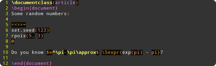
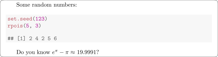
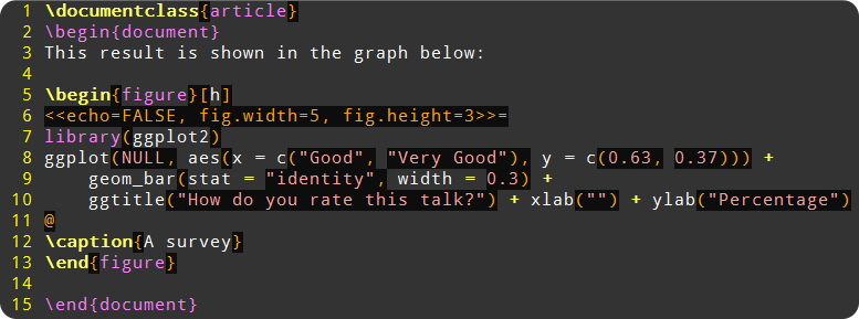
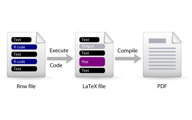
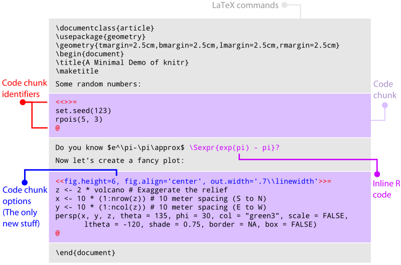
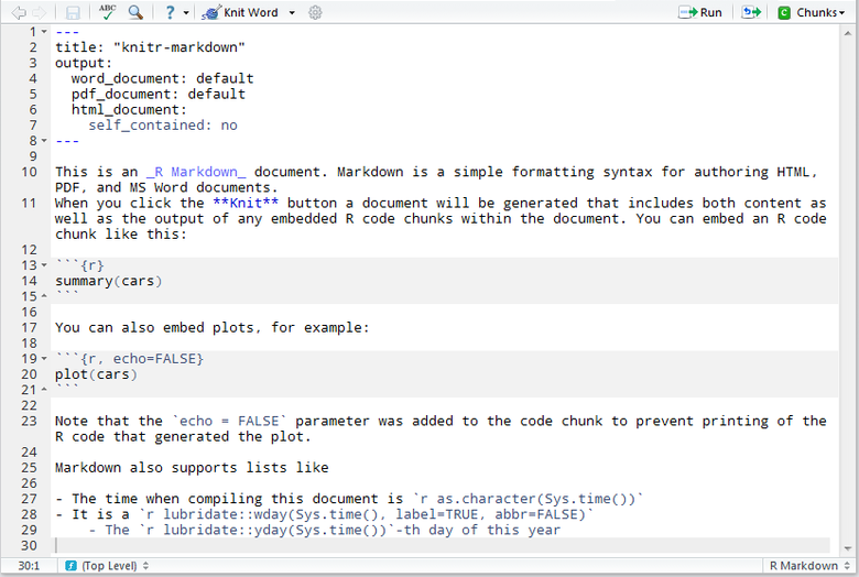
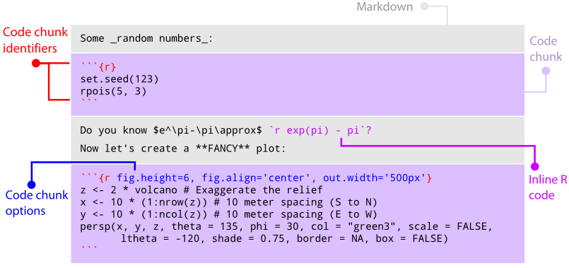
  • Human language and code in the same document
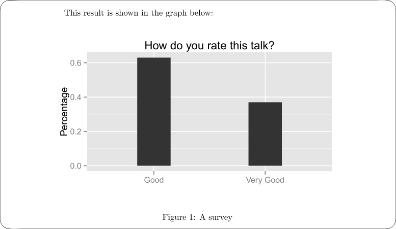
  • Code can be excuted and replaced by its output
  • Focus more on content, less on format

A minimal example

Source code

After compiling

A minimal example (plots)

Source code

A minimal example (plots)

After compiling

Basic idea

Tools

Early stage – Sweave

  • To "weave" S
  • Developed by R Core, very powerful

Today – knitr

Structure

Most useful options (output)

  • Default option, show both source code and output
<<>>=
x <- seq(1, 6, by = 0.5)
x
sin(x)
@
  • Show R source code only
<<eval=FALSE>>=
@
  • Show code output only
<<echo=FALSE>>=
@

Most useful options (output)

  • Whether to format the code or not
<<tidy=FALSE>>=
x<-                 seq(1,6,
    by=0.5)
x
@
  • Only evaluate the code, do not show anything. Mainly used to create variables for later use.
<<include=FALSE>>=
dat = rnorm(100)
@

Most useful options (plot)

  • Figure width and height (in R side)
<<fig.width=6, fig.height=6>>=
plot(density(dat))
@
  • Figure width and height (in output document side)
<<out.width='0.7\\textwidth'>>=
plot(density(dat))
@
  • Alignment and caption
<<fig.align='center', fig.cap="A density plot">>=
plot(density(dat))
@

From \(\LaTeX\) to Markdown

\(\LaTeX\) is a powerful language to write document, but…

  • Not easy to get started
  • Complicated, typing too many commands
  • Restricted output file format (mainly for PDF)

Another friend of knitr – Markdown

  • So… another language to learn?
  • Yes, but…
  • Much, much, much easier than \(\LaTeX\)
  • Can be converted into \(\LaTeX\), HTML, Word etc.

An overview of Markdown+knitr

Markdown basics

  • Headers
## Methodology 
In this section we introduce our methodology.

### Algorithm
The algorithm is blablabla...

### Simulation
Now we show our simulation result.
  • Similar to \section{} and \subsection{} in \(\LaTeX\)

Markdown basics

  • Decorations (bold, italic, etc.)
You should **NEVER** claim to _accept_ a null hypothesis

You just say **_do not reject_**
  • Rendered result

You should NEVER claim to accept a null hypothesis

You just say do not reject

Markdown basics

  • Code
There is some inline code: `print(x)`

And code blocks:
```
x <- rnorm(100)
summary(x)
```
  • Rendered result

There is some inline code: print(x)

And code blocks:

x <- rnorm(100)
summary(x)

Markdown basics

  • Math formulas
The series $\sum_i \frac{1}{n}$ is divergent, i.e.,
$$\sum_i \frac{1}{n}=\infty$$
  • Rendered result

The series \(\sum_i \frac{1}{n}\) is divergent, i.e.,

\[\sum_i \frac{1}{n}=\infty\]

Markdown basics

  • Item lists
There are three kinds of lies:

- Lies
- Damned lies
- Statistics
    - Frequentists
    - Bayesian

There are three kinds of lies:

  • Lies
  • Damned lies
  • Statistics
    • Frequentists
    • Bayesian

Markdown basics

  • Links and images
[A 5-minute tutorial of Markdown](http://goo.gl/JqhpOf)

The talk is boring, but please wake up! ![](images/tuzki31.gif)
  • Rendered result

A 5-minute tutorial of Markdown

The talk is boring, but please wake up!

knitr with Markdown

More expressive, more impressive

  • 3-D interactive plots
  • Animation
  • Slides
    • Did I tell you this slide was written using Markdown+knitr?
  • More data analysis reports at RPubs
  • More visualization examples at Vistat

Resources

Acknowledgement

Thanks to Yihui Xie, the creator of knitr, for creating this wonderful tool, and for providing me lots of help in using knitr.

Thanks for your patience!

Questions?