Beyond Bayes: What We Can Do with a Partial Prior

class: center, middle, inverse, title-slide

# Beyond Bayes: What We Can Do with a Partial Prior
## @ GSO Seminar
### Yixuan Qiu
### 04/06/2017<br/><br/>Joint work with Prof. Lingsong Zhang and Chuanhai Liu

---

# Outline

- Prologue — About Bayes
- Motivation — A Partial Prior
- Problem — Partially Specified Bayesian Models
- Foundation — The Inferential Models
- Methodology — The Partial Bayes Method
- Application — NBA Three-Point Shots

---
class: inverse, center, middle

# Prologue

---

# A Picture I Took Today at HAAS

![](images/posters.jpg)

---

# A Closer Look...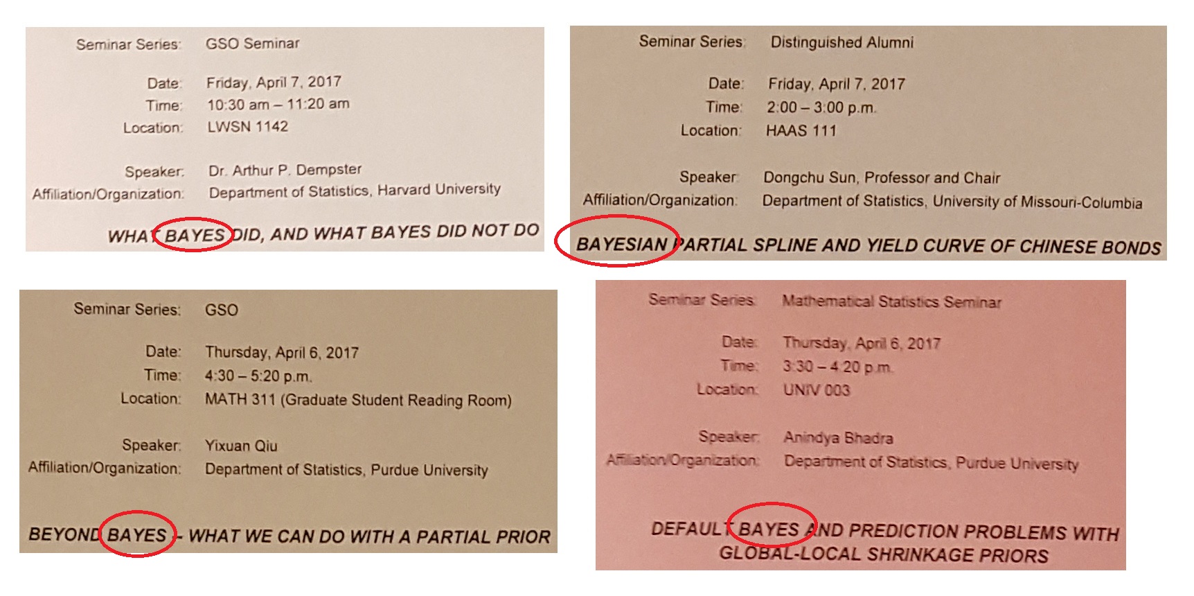

![](images/posters3.jpg)

---

# About Bayes

- Bayes' Theorem provides a great framework for statistical inference
- Knowledge = Prior + Data

![](images/bayes.jpg)

---

# Bayesian Procedure

- Interested in parameter `$\theta$`
- Prior: `$\pi(\theta)$`
- Data: `$f(x|\theta)$`
- .emph[Posterior]

`$$q(\theta|x)=\frac{\pi(\theta)f(x|\theta)}{\int \pi(\theta)f(x|\theta) \mathrm{d}\theta}$$`
--

- What if `$\pi(\theta)$` is .warning[NOT] known?
--

- What if `$\pi(\theta)$` is .warning[partially] known?

---
class: inverse, center, middle

# Motivation

---

# A Partial Prior

- Consider a normal hierarchical model
- There are `$n$` groups of data, mutually independent, each with group mean `$\mu_i$`
- Observation in each group is `$X_i|\mu_i\sim N(\mu_i,1)$`
- The group means have a common prior `$\mu_i\sim N(\mu,1)$`
- We are interested in `$\mu_1$`, and want to construct an interval estimation
- However, `$\mu$` is .warning[unknown]

---

# A Partial Prior cont.

- A diagram of partial prior

![](images/pb_diagram.png)

---

# Some Attemps

- Frequentist: `$X_1-\mu_1\sim N(0,1)$`
--

- .warning[Totally ignore the information from prior and other groups]
--

- Bayes: `$\mu_1|\{X_1,\ldots,X_n\}\sim N\left(\frac{1}{2}X_1+\frac{1}{2}\mu,\frac{1}{2}\right)$`
--

- .warning[
Cannot proceed since `$\mu$` is unknown
]
--

- Empirical Bayes: `$\hat{\mu}=\bar{X}$`, `$\mu_1|\{X_1,\ldots,X_n\}\overset{approx}{\sim} N\left(\frac{1}{2}X_1+\frac{1}{2}\bar{X},\frac{1}{2}\right)$`
--

- .warning[Uncertainty quantification is inaccurate]

---
class: inverse, center, middle

# Problem

---

# Partially Specified Bayesian Model

- Parameter `$\theta$` is partitioned into two blocks `$\theta=(\tilde{\theta},\theta^{*})$`
- If prior is fully given, `$\pi_0(\theta)=\pi(\tilde{\theta}|\theta^{*})\pi^{*}(\theta^{*})$`
- .emph[
In PB models, only `$\pi(\tilde{\theta}|\theta^{*})$` is available
]

<table class="table">
  <tr>
    <td>Sampling Model</td>
    <td>$X|\theta\sim f(x|\theta)$</td>
  </tr>
  <tr>
    <td>Parameter Partition</td>
    <td>$\theta=(\tilde{\theta},\theta^{*})$</td>
  </tr>
  <tr>
    <td>Partial Prior</td>
    <td>$\tilde{\theta}|\theta^{*}\sim\pi(\tilde{\theta}|\theta^{*})$</td>
  </tr>
  <tr>
    <td>Component without Prior</td>
    <td>$\theta^{*}$</td>
  </tr>
  <tr>
    <td>Parameter of Interest</td>
    <td>$\eta=h(\tilde{\theta})$</td>
  </tr>
</table>

---

# Inference Tools for PB Models

- PB models reside in the "middle" of Bayes and Frequentist
- Neither of these two is ideal to tackle such problems
- We need new tools and techniques to do the inference
- The .emph[Inferential Models] theory (Martin and Liu, 2013) provides
a promising framework for PB models

---
class: inverse, center, middle

# Foundation

---

# The Inferential Models

The Inferential Modles (IMs) framework is:

- A new paradigm for statistical inference
  - .emph[Parallel to Bayesian and Frequentist]
- Compatible with Bayesian and Frequentist
  - .emph[Able to reproduce the results by these two]
- Designed for exact inference
  - .emph[Interval estimators have guaranteed coverage probability]
--

- Was born in Purdue Statistics!

---

# The IM Procedure

IM has a three-step procedure for inference:

- .emph[Association]: Connects the parameter, observed data, and
unobserved auxiliary random variable through an association function
- .emph[Prediction]: Uses a random set to predict the unobserved
auxiliary random variable
- .emph[Combination]: Transform the uncertainty from the auxiliary
space to the parameter space
--

- .warning[Don't panic — I will give examples shortly]

---

# The IM Outputs

IM has two output quantities:

- The .emph[belief] function: Quantifies how much evidence supports that an assertion is true, and
  - .emph["Direct" evidence]
- The .emph[plausibility] function: Quantifies how much evidence does not support that an assertion is false
  - .emph["Indirect" evidence]

---

# A Simple Example

Given `$X\sim N(\theta, 1)$`, want to do inference on `$\theta$`
--

- A-step: `$X=\theta+Z,\ Z\sim N(0,1)$`
--

- P-step: Use a random interval `$\mathcal{S}=(-|V|,|V|),\ V\sim N(0,1)$` to
predict the true value of `$Z$`
--

- C-step: Since `$\theta=X-Z$`, given the observed data `$x$`, we use
`$\Theta_x(\mathcal{S})=(x-|V|,x+|V|)$` to cover `$\theta$`

---

# A Simple Example cont.

For any assertion on `$\theta$`, for example `$A=\{\theta: 1<\theta<2\}$`

- Belief:
`$$\begin{align*}
\mathsf{bel}_{x}(A) & =P\{\Theta_{x}(\mathcal{S})\subseteq A|\Theta_{x}(\mathcal{S})\ne\varnothing\}\\
 & =P\{x-|V|>1,x+|V|<2\}
\end{align*}$$`
- Plausibility: `$\mathsf{pl}_{x}(A)=1-\mathsf{bel}_{x}(A^{c})$`
- .emph[Plausibility Interval]: `$\mathsf{PR}_{x}(\alpha)=\{\theta:\mathsf{pl}_{x}(\{\theta\})>\alpha\}$`
  - Comparable to Bayesian credible interval and Frequentist's confidence interval

---

# Extensions of IMs

- Marginal IM: Dealing with nuisance parameters
- Conditional IM: Combining information

A Bayesian example: `$\theta\sim Exp(1),\ X,Y|\theta\overset{indep}{\sim} N(\theta,1)$`

- Association
`$$\begin{cases}
\theta=e\\
X=\theta+Z_{1}\\
Y=\theta+Z_{2}
\end{cases}\Rightarrow\begin{cases}
\theta & =e\\
X & =e+Z_{1}\\
X-Y & =Z_{1}-Z_{2}
\end{cases}$$`
- `$e+Z_1$` and `$Z_1-Z_2$` are fully observed
- Use `$e|\{e+Z_1=x,Z_1-Z_2=x-y\}$` to predict `$e$`

---
class: inverse, center, middle

# Methodology

---

# The Partial Bayes Method

- Using IMs to solve PB models
- Recall the partial prior example with `$n=2$`

`$$\mu_1,\mu_2\overset{indep}{\sim}N(\mu,1),\ X_i|\mu_i\overset{indep}{\sim} N(\mu_i,1),\ i=1,2$$`

- Association
`$$\begin{cases}
X_{1}=\mu_{1}+e_{1}=(\mu+\varepsilon_{1})+e_{1}\\
X_{2}=\mu_{2}+e_{2}=(\mu+\varepsilon_{2})+e_{2}
\end{cases}\Rightarrow\begin{cases}
X_{1} & =\mu_{1}+e_{1}\\
X_{2}-X_{1} & =\varepsilon_{2}-\varepsilon_{1}+e_{2}-e_{1}
\end{cases}$$`

- Use `$e_1|\{\varepsilon_{2}-\varepsilon_{1}+e_{2}-e_{1}=x_2-x_1\}\equiv N\left(\frac{1}{4}(x_{1}-x_{2}),\frac{3}{4}\right)$` to predict `$e_1$`

---

# The Normal Hierarchical Model

- Generally, for `$X_{i}|\mu_i\sim N(\mu_{i},\sigma^{2})$`, `$\mu_{i}\sim N(\mu,\tau_{0}^{2})$` where `$\sigma^2$` and `$\tau_0^2$` are known constants, the plausibility interval for `$\mu_1$` is
`$$\frac{\tau_{0}^{2}}{\tau_{0}^{2}+\sigma^{2}}X_{1}+\frac{\sigma^{2}}{\tau_{0}^{2}+\sigma^{2}}\overline{X}\pm z_{\alpha/2}\sigma\sqrt{1-\frac{n-1}{n}\cdot\frac{\sigma^{2}}{\tau_{0}^{2}+\sigma^{2}}}$$`

![](images/eb_pb.png)

---

# Other Studied Models

- Normal hierarchical model in which both parameters in the prior are unknown
- Poisson hierarchical model (used in the application part)
- Two sample binomial model: `$X\sim B(m,p_1),\ Y\sim B(n,p_2)$`, prior is on
`$\delta=p_1-p_2\sim \pi(\delta)$`, and we want to do inference on `$\delta$`

---
class: inverse, center, middle

# Application

---

# Basketball Three-Point Shot

.left69[
- Rewards the highest score in one single attempt
- Valuable for a team that has very limited offensive possessions
- The choice of player that will make the attempt is crucial
- .emph[How to evaluate shooter's performance?]
]

.right30[
![](images/three_point_shot.jpg)
]

???

Image credit: http://m.bizhizu.cn/pic/1471.html
---

# NBA Three-Point Shooters Data

- Data obtained from the official NBA website
- 2015-2016 regular season
- Select three players from each team
- Retrieve data from each player's last ten games within the season

---

# Overview of Data Set

<div id="htmlwidget-99e7ede6f7f16f13b796" style="width:100%;height:auto;" class="datatables html-widget"></div>
<script type="application/json" data-for="htmlwidget-99e7ede6f7f16f13b796">{"x":{"filter":"none","data":[["Dirk Nowitzki","Mike Miller","Joe Johnson","Mike Dunleavy","Luis Scola","David West","Matt Bonner","Kyle Korver","J.R. Smith","Trevor Ariza","Chris Paul","Ersan Ilyasova","Lou Williams","Jose Calderon","JJ Redick","Kyle Lowry","Steve Novak","Jose Juan Barea","Kevin Durant","Jared Dudley","Arron Afflalo","Carl Landry","Marc Gasol","D.J. Augustin","Jerryd Bayless","George Hill","Darrell Arthur","James Harden","Stephen Curry","Tyler Hansbrough","Jeff Teague","Darren Collison","Omri Casspi","Toney Douglas","Jonas Jerebko","Jodie Meeks","Patrick Beverley","Paul George","Luke Babbitt","Avery Bradley","Nemanja Bjelica","Lance Stephenson","Donald Sloan","Gary Neal","Lance Thomas","Enes Kanter","Klay Thompson","Alec Burks","Kawhi Leonard","Bojan Bogdanovic","Justin Harper","Chandler Parsons","Jon Leuer","E'Twaun Moore","Michael Kidd-Gilchrist","Bradley Beal","Meyers Leonard","Andrew Nicholson","Evan Fournier","Khris Middleton","Mike Scott","Hollis Thompson","Mirza Teletovic","Allen Crabbe","CJ McCollum","Isaiah Canaan","Kelly Olynyk","Reggie Bullock","James Ennis","Matthew Dellavedova","Raul Neto","Seth Curry","Troy Daniels","Jordan McRae","Zach LaVine","Jordan Clarkson","CJ Wilcox","Glenn Robinson","Doug McDermott","TJ Warren","James Michael McAdoo","Josh Huestis","Tyler Johnson","Xavier Munford","D'Angelo Russell","Karl-Anthony Towns","Trey Lyles","Norman Powell","Josh Richardson","Darrun Hilliard"],["DAL","DEN","MIA","CHI","TOR","SAS","SAS","ATL","CLE","HOU","LAC","ORL","LAL","NYK","LAC","TOR","MIL","DAL","OKC","WAS","NYK","PHI","MEM","DEN","MIL","IND","DEN","HOU","GSW","CHA","ATL","SAC","SAC","NOP","BOS","DET","HOU","IND","NOP","BOS","MIN","MEM","BKN","WAS","NYK","OKC","GSW","UTA","SAS","BKN","BKN","DAL","PHX","CHI","CHA","WAS","POR","ORL","ORL","MIL","ATL","PHI","PHX","POR","POR","PHI","BOS","DET","NOP","CLE","UTA","SAC","CHA","CLE","MIN","LAL","LAC","IND","CHI","PHX","GSW","OKC","MIA","MEM","LAL","MIN","UTA","TOR","MIA","DET"],[52,13,38,22,38,2,17,47,73,60,36,18,52,29,54,73,15,53,81,13,28,6,0,36,36,36,30,91,117,0,38,26,23,48,18,9,48,62,33,45,24,14,16,18,21,6,82,17,43,52,9,55,10,24,7,48,34,29,49,34,23,71,82,36,56,74,26,18,52,26,14,59,38,7,53,58,13,9,16,13,2,6,17,19,42,22,41,38,33,15],[14,5,11,7,19,1,6,16,31,23,11,7,19,12,22,24,7,22,31,4,9,4,0,13,16,16,11,42,54,0,16,13,9,21,7,4,20,22,16,16,14,8,6,5,7,4,30,9,15,20,4,24,4,12,3,17,18,12,19,11,10,28,28,17,26,25,11,7,24,7,3,29,16,5,20,17,6,5,5,5,1,4,5,8,15,7,17,21,13,6],["26.92%","38.46%","28.95%","31.82%","50.00%","50.00%","35.29%","34.04%","42.47%","38.33%","30.56%","38.89%","36.54%","41.38%","40.74%","32.88%","46.67%","41.51%","38.27%","30.77%","32.14%","66.67%","NaN%","36.11%","44.44%","44.44%","36.67%","46.15%","46.15%","NaN%","42.11%","50.00%","39.13%","43.75%","38.89%","44.44%","41.67%","35.48%","48.48%","35.56%","58.33%","57.14%","37.50%","27.78%","33.33%","66.67%","36.59%","52.94%","34.88%","38.46%","44.44%","43.64%","40.00%","50.00%","42.86%","35.42%","52.94%","41.38%","38.78%","32.35%","43.48%","39.44%","34.15%","47.22%","46.43%","33.78%","42.31%","38.89%","46.15%","26.92%","21.43%","49.15%","42.11%","71.43%","37.74%","29.31%","46.15%","55.56%","31.25%","38.46%","50.00%","66.67%","29.41%","42.11%","35.71%","31.82%","41.46%","55.26%","39.39%","40.00%"]],"container":"<table class=\"display\">\n  <thead>\n    <tr>\n      <th>player<\/th>\n      <th>team<\/th>\n      <th>attempted<\/th>\n      <th>made<\/th>\n      <th>percentage<\/th>\n    <\/tr>\n  <\/thead>\n<\/table>","options":{"columnDefs":[{"className":"dt-right","targets":4},{"className":"dt-right","targets":[2,3]}],"order":[],"autoWidth":false,"orderClasses":false}},"evals":[],"jsHooks":[]}</script>

---

# Estimate Success Rate

- Point estimator: `$\hat{p}_{i}=X_{i}/n_{i}$`, `$X_i$` is the number of three-point shots made in `$n_i$` attemps by player `$i$`
--

- .emph[How to quantify the uncertainty? 1/5 v.s. 10/50]
- .emph[Any other assumptions we can make to improve the estimator?]
--

- Players in the league may share some common characteristics
  - `$X_i|p_i\sim Pois(n_i p_i)$`
  - `$p_i\sim Exp(\theta)$`
  - We leave `$\theta$` unspecified
  - Do inference on `$p_i$`

---

# Results

![](images/nba.png)

---

# Results

![](images/players.png)

---

# Summary

- The partial prior problem calls for methodology beyond Bayes
- We formalize such problems to introduce the Partially Specified Bayesian Models
- Based on the Inferential Models theory, we develop the Partial Bayes method
to solve PB models
- Partial Bayes method provides exact inference results for any finite sample
size

---
class: inverse

# Acknowledgement

- I would like to thank Prof. Lingsong Zhang and Chuanhai Liu for their invaluable supervising
- Thank Yaowu Liu for the extensive discussions on the IM theory
- Thank Zach Hass and Nathan Hankey for their great help in the basketball example
- Thank Will Eagan for organizing the GSO seminar
- Thank the audience coming today